 feint labs
Inside Chessformer: predicting the move a person will play
In this article
Put a tempting capture in front of ten chess players and you may get several different replies. Some will take it. Some will see the problem. Someone will find a perfectly legal move you hadn't considered.
For Feint, predicting that spread is useful. The move selector needs probabilities over human replies to judge which opportunities are worth creating. A list of engine-approved moves answers a different question.
We give the model recent boards as well as the current one. A player may still be following a plan from a turn ago. A capture just offered can also shape their next move. We include information about the player and game too. A beginner playing blitz has less time and experience than a strong player in a classical game. At a high level, our player model takes three things—recent board history, player and game context, and the set of legal moves—and outputs a probability distribution over what the person across the board will play next.
Our predictor is an independent, scaled-down implementation of Chessformer, an architecture introduced by Daniel Monroe and colleagues. Some earlier models read a list of PGN moves. Others put board squares in a single row. Neither layout follows the paths of bishops or knights very well. Chessformer gives each square its own token, with recent board history. It adds board geometry through Geometric Attention Bias and scores moves by comparing origin and destination squares directly. The paper reports better human-move prediction with far fewer parameters and less compute.
That efficiency is what makes a live browser model possible. The version used in Feint Chess has about 1.4 million parameters, eight transformer blocks, four attention heads and a hidden width of 128.
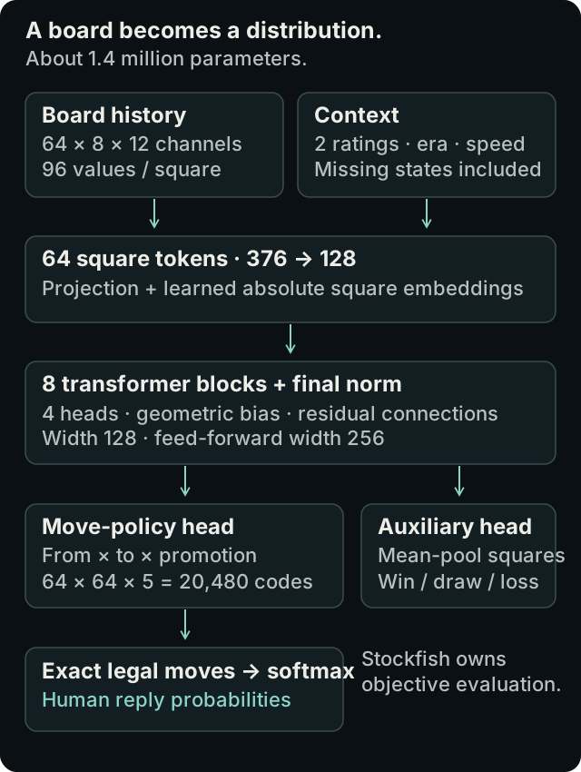
Sixty-four tokens, not a sentence of moves
Rather than feeding the transformer a sequence of past moves or 512 separate space-time tokens (), we feed it just 64 square tokens—each carrying its own eight-position history.
Getting the board representation into its present form took quite a bit of trial and error. The diagram, conveniently, only has to show the version we kept: eight snapshots (the current board and seven earlier positions, one half-move apart) that show how the position developed.
Each token belongs to one square and tracks occupancy across all eight snapshots using twelve binary channels (six piece types for the mover, six for the opponent, or all zeros when empty):
Every snapshot is oriented from the current mover's perspective. When it's Black's turn, all eight frames are rotated 180 degrees and channels are swapped so the model always sees 'my pieces' versus 'their pieces.' Early in the game, when fewer than eight snapshots exist, we pad the history by repeating the initial board.
The input is also deliberately incomplete as a full chess state. Piece history alone doesn't always determine castling rights or repetition status. The rules layer owns legality and supplies the legal move codes. The neural model doesn't get to decide that an illegal castle would be popular today.
Context travels with every square
An offer that fools a 1200-rated player may be no use against a 2400-rated one. Time to think can change that choice too. To account for this, mover rating, opponent rating, era and game speed are attached to every square before the transformer blocks begin.
For ratings, we blend two learned endpoints across a 0–5000 scale:
Because the network is nonlinear, a 60:40 mix of rating inputs (for ) doesn't just produce a naive 60:40 average of move probabilities. We can query the same trained network at any rating, or blend several rating conditions at once during live play, as described in the S1 article. Missing ratings have their own learned states rather than defaulting to an average player.
The era input covers modern play and five historical bands. Speed can be blitz, rapid, classical or unknown. Each has a small learned vector, called an embedding. We join these with the square's 96 history values. A linear projection maps that input to 128 features. We also add a vector learned for each square. This tells the model that empty e1 and empty e8 are different places.
Attention: which squares should exchange information?
Unlike an autoregressive language model, there is no causal mask hiding 'future' squares—and distance on the board is no barrier, so e1 can talk straight to e8 in layer one.
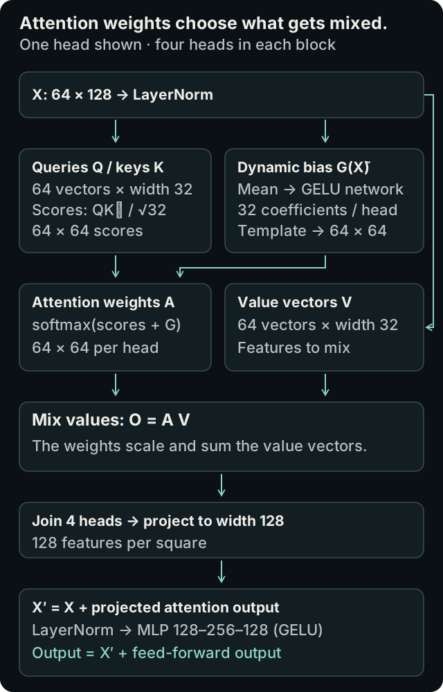
Within each attention head, every normalized square token () produces a query, a key and a value vector of 32 numbers. Value vectors carry the features passed between squares; they are not chess evaluations.
To help the heads learn board geometry without hardcoding rules, we add a Geometric Attention Bias () to the query-key scores before normalizing them into attention weights:
The branch starts by averaging the block's normalized tokens into a compressed view of the board and passing it through a small network to produce 32 coefficients per head ():
The table has one bias for each pair of squares. Its 4,096 entries are built from those 32 coefficients. Every layer and head uses the same learned template. Its weights stay fixed after training. The coefficients change with the board, so the bias changes with the position.
Averaging the tokens saves work in the bias branch, while the individual square details still flow intact through the queries, keys and values.
From Squares to Legal Moves
Instead of predicting moves from a single pooled board vector, the policy head scores each move by directly comparing its origin square to its destination square.
After the eighth transformer block, each square has a final representation . Take e2–e4. We project e2's vector with and e4's with . Their scaled dot product is the base score:
Promotions add a learned bias to this score. We reserve five slots for every square pair (no promotion, plus knight, bishop, rook, and queen), yielding possible move codes—most of which are gloriously impossible in any single position.
Before running softmax, the rules layer filters those 20,480 codes down to the strictly legal moves. Illegal moves are barred at the door; legal but dreadful moves are warmly invited in, since humans do play them.
What the Loss Function Actually Rewards
Training examples pair a position and context with the move a human actually played. Our main loss is negative log-likelihood. We average it over examples in a batch:
Suppose the model gave the human's move a 25% chance. Its loss on that example is nats. Assigning higher probability to that move lowers the loss—even if the move is a catastrophic blunder that makes Stockfish weep. Our job here is to predict the human, not fix their chess.
We also include a lightly weighted () auxiliary head that predicts the game's win/draw/loss result from the pooled square vectors. This gives the shared representation an extra training signal, though Stockfish still owns all objective evaluation during actual gameplay.
For chess research data, we credit Lichess for standard positions and Oden-worldchess for historical games.
We trained for 500,000 steps at a batch size of 4,096—over 2 billion positions in total. Across roughly half a million development positions, the model's top choice matched the human's actual move 56.6% of the time, with a post-training temperature calibration step to keep the full probability distribution well-scaled for the S1 selector.
From Trained Weights to Browser Gameplay
To keep the download small, we ship large weight matrices as scaled INT8 values and reconstruct them as floating-point weights in the browser—so compact storage doesn't require integer matrix kernels at runtime. Inference runs inside a WebAssembly worker using 4-wide SIMD instructions to speed up attention dot products (with a scalar fallback for browsers without SIMD). We’ll cover our browser optimization tricks—along with our sister models for checkers (Draughtsformer) and Othello (OthelloFormer)—in upcoming posts.
At the end of that path, the output is still a distribution over legal moves. The move selector has to turn that information into an opponent worth playing. A more accurate predictor doesn't settle that question. Computers are quite capable of being correct and tedious at the same time.
The S1 article explains how the resulting reply distribution participates in a move decision.